In many markets prices don't change much, even when supply or demand change. The price of the Wall Street Journal doesn't rise just because a popular story increases demand on a particular day. Taxis don't increase their fares when it rains heavily and demand suddenly goes up. Hotels don't vary room rates in response to daily fluctuations in demand. Firms seldomly cut wages when sales fall. When prices don't react quickly to changes in supply and demand economists say that 'prices are sticky'.

Of course, in many markets prices do adjust quickly to shifts in supply or demand. Think for instance of markets for fresh food, markets for commodities such as oil, or money markets (where the prices are interest rates). However, in markets where demand and supply are highly variable, but prices are constrained to move more slowly, there is an inefficiency in the market.

Eliminating inefficiencies in existing markets is what many internet enterprises are about (as well as creating new products). Much has been written about how dot.com firms have reduced the transaction costs of bringing buyers and sellers together. But the potential of the internet to increase the efficiency of markets by making prices less sticky has received little attention. Understanding how internet enterprises can create value by reducing price stickiness in existing markets is the subject of the next article in this issue of Paradigm.

Price flexibility in a single market
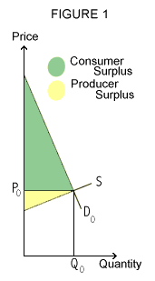
The relationship between price flexibility and economic efficiency is illustrated in the simple supply and demand diagrams of Figures 1, 2 and 3. Figure 1 shows an initial market equilibrium where the market price and quantity sold is (P0,Q0). The supply curve is upward sloping. Think for instance of the trucking industry. The number of trucks is fixed in the short run, but in periods of high demand haulage rates rise, and in response drivers work longer hours which increases the supply of haulage to meet the higher demand. Figure 1 also shows consumer surplus and producer surplus.

Case with no price stickiness
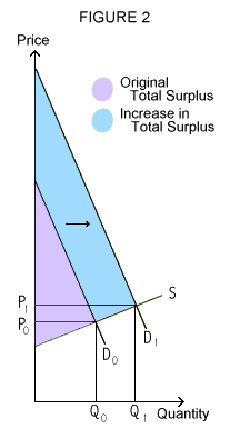
Imagine that there is no price stickiness in the trucking industry and that the demand for freight haulage rises. Figure 2 illustrates. The increased demand is represented by a shift of the demand curve to the right. At every price of haulage the amount demanded has increased. Demand exceeds supply at the original price P0. The excess demand is then completely resolved by an increase in price to P1. As price goes up supply increases. Moreover, as the price increases the buyers who receive the least benefit from haulage services find that the price now exceeds their valuation. In that way the price rise ensures that when the market adjusts to the increase in demand the market output goes to the buyers who value that output the most. The rising price increases supply and reduces demand until the new equilibrium at (P1,Q1) is reached.

Figure 2 also shows the increase in total surplus (consumer surplus plus producer surplus). How is the increase in surplus divided between producers and consumers? That depends upon the relative steepness of the supply and demand curves. If demand is more inelastic (steeper sloped) than supply, then more of the increase in surplus will go to the buyers than to the sellers. Saying that demand is inelastic is the same as saying that there are no close substitutes for truck haulage.

Note that Figure 2 really shows the short run situation, because in the long run we should expect that the increased industry profits will lead to new trucking firms entering the industry and existing firms expanding. In that case the supply curve is probably close to horizontal in the long run.

Introducing price stickiness
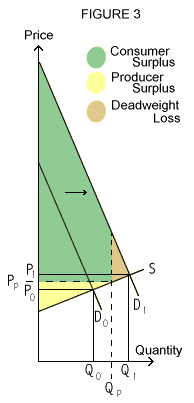
Now imagine that demand increases but prices cannot fully adjust to clear the market, or that prices adjust very slowly. Figure 3 shows the case of partial adjustment where price increases from P0 to Pp . Output then only rises from Q0 to Qp. So the price increase can only partially resolve the excess demand created by the shift of the demand curve. The deadweight loss is the loss of total surplus that is caused by the inability of prices to fully adjust. It arises because for every unit of output between Qp and Q1 there is a buyer would be prepared to pay more than the marginal cost of production. This is an output level inefficiency. If the price could rise from Qp to Q1 then the total surplus could increase by the amount of the deadweight loss.

If prices can fully adjust then no problem. But if prices are sticky then the resulting loss of surplus is deadweight loss. So if we could costlessly eliminate the price stickiness, then we would create value (increase total surplus) equal to the deadweight loss.

Figure 3 actually shows only the minimum loss of surplus arising from price stickiness and understates the potential gains from making prices more flexible. It is assumed in Figure 3 that, despite the excess demand, the supply ends up with the buyers who put the highest value on the product. But it is price adjustment itself that causes the output to go to the buyers who most highly value it. If the price stickiness causes some output to go to buyers who have lower valuations than others that miss out, then there is an allocation inefficiency which makes total inefficiency greater than shown in Figure 3.

When is price stickiness most important?
When demand increases and the market goes from one equilibrium to another, both price and quantity change. If most of the change between one equilibrium and another is in quantity rather than price then price stickiness will not be important. When does that happen? When either the supply or demand curves are highly elastic (have small slopes). Equivalently we can say that efficiency gains from reducing price stickiness will be found in markets where either demand or supply is inelastic and neither is highly elastic.

Taxi cab example
Consider an example to illustrate allocation inefficiency and output level inefficiency. In some cities a cab license can be issued to any person of good character who has a suitable motor vehicle. Say that the one time license fee is $25,000, but the price is fixed at $2 per mile. Then owners will offer their cabs when demand for cab rides is expected to be high and withdraw when demand is low. So demand and supply will be about equal.

Sometimes, however, there will be unexpectedly high demand, such as when it rains heavily. If prices were fully flexible then they would rise until customers with low valuations of a taxi ride were squeezed out and those with the highest valuations of a taxi ride got to ride. But instead, prices are fixed. So in the face of excess demand the allocation may be essentially random, and consequently there is allocation inefficiency. This is economically inefficient because a passenger with a low valuation could receive a side payment to give up her taxi ride to someone who would pay more, and both could then be better off. (One of three requirements for economic efficiency is that all buyers must have the same marginal value of the product).

You might think then that introducing price flexibility only benefits the cab owners and wealthier customers who get cabs when cabs are scarce, albeit at a higher price. However, that ignores the product level inefficiency. If cab drivers can get more revenues because the price is higher during demand spikes then the number of cabs will increase and prices will decrease for the times when there is no demand spike. If you have low valuation of cabs and only ever take a cab when it rains, then you are certainly worse off if prices become flexible, but in aggregate society is better off with a more optimal allocation and production level.

Next Page