Overview of the Sensitivity Toolkit
The Sensitivity Toolkit was created to bring the most powerful tools of sensitivity analysis to the spreadsheet. The Toolkit supports four different forms of sensitivity analysis:
Data Sensitivity creates a table and chart to show how an output cell varies with changes in one (or two) inputs. In Tornado Chart, a set of parameters is varied from low to high and the results for a single output cell are reported. Solver Sensitivity runs the optimization program Solver on a spreadsheet for a set of values for one (or two) parameters. Similarly, Crystal Ball Sensitivity runs the simulation program Crystal Ball on a spreadsheet for a set of values for one (or two) parameters.
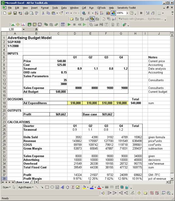
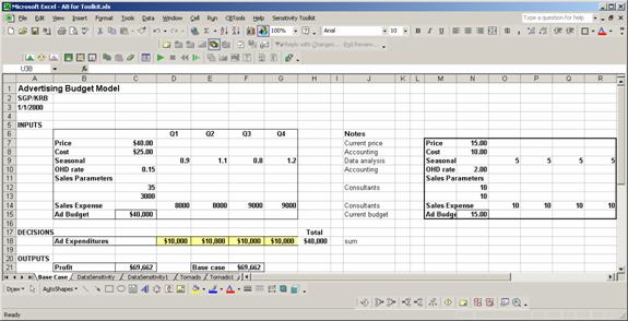
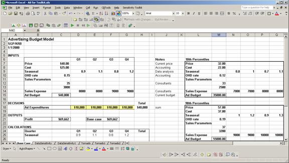
This document illustrates how each of these tools works. We will use the spreadsheet Advertising Budget Model.xls (shown below) to illustrate the various options.
Purpose: Data Sensitivity is used to trace the effect on an output of changes in one (or two) inputs.
Options:
One-way table: specify one input parameter
Two-way table: specify two input parameters
Examples:
One-way table
Question: How sensitive is Profit to changes in the Price?
Procedure:
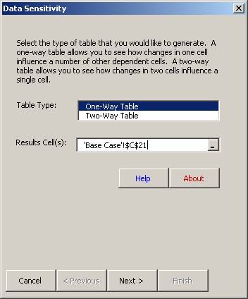
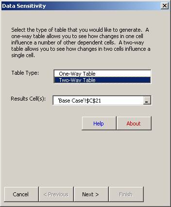
Select Sensitivity Toolkit – Data Sensitivity.
Select One-Way Table and specify the cell address for the Result, in this case Profit in cell C21.
Click on Next.
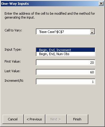
Specify the Cell to Vary, Price, in C7.
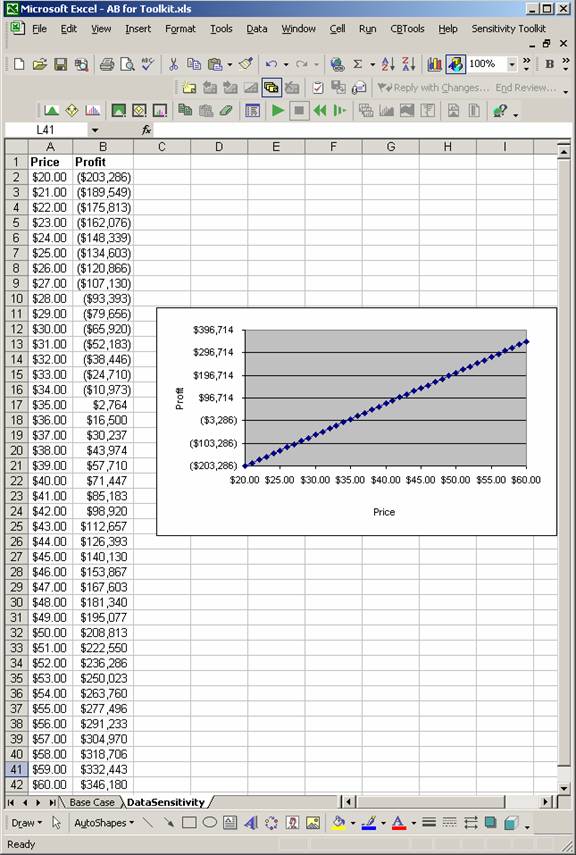
Choose the range of prices, from 20 to 60 in steps of 1.
Click on Finish.
The results consist of a table showing the Profit resulting for each value of Price. A line chart is automatically generated from this table.
Two-way table
Question: How sensitive is Profit to changes in the Price and in the Cost?
Procedure:
Select Sensitivity Toolkit – Data Sensitivity.
Select Two-Way Table and specify the cell address for the Result, in this case Profit in cell C21. (Note: Two-way tables may have only one Result cell specified.)
Click on Next.
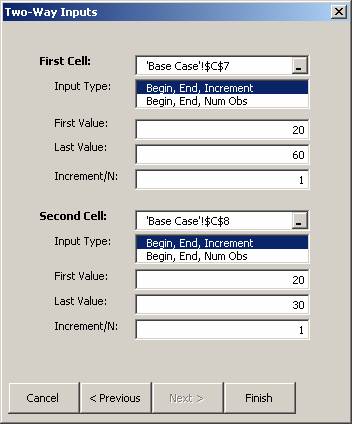
Specify the First Cell to vary, Price, in C7.
Choose the range of prices, from 20 to 60 in steps of 1.
Specify the Second Cell to vary, Cost, in C8.
Choose the range of prices, from 20 to 30 in steps of 1.
Click on Finish.
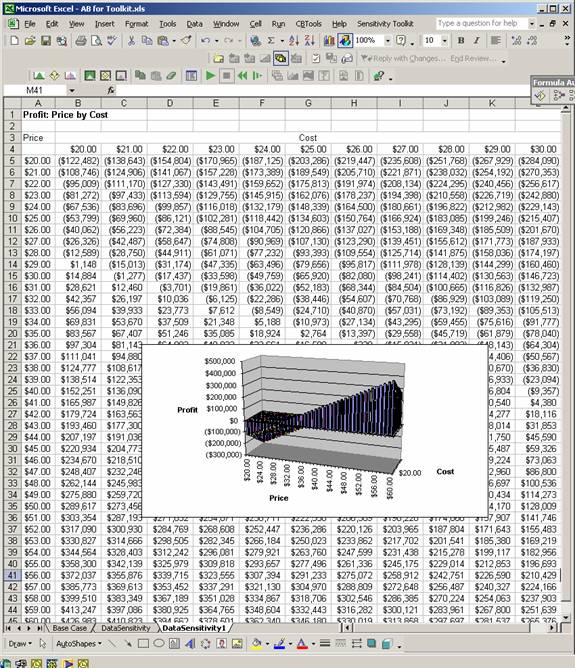
The results consist of a table showing the Profit resulting for each value of Price and Cost. A 3D chart is automatically generated from this table.
Purpose: A Tornado Chart ranks input parameters in terms of their impact on the output. This tool allows the user to create Tornado Charts for a spreadsheet using one of three alternative approaches. It provides a convenient way to determine the relative sensitivity of the results to an entire set of input parameters.
Options:
1. Common Percentage Option: varies each parameter up and down by the same percentage of the base case value.
2. Variable Percentage Option: varies each parameter up and down by its own percentage of the base case.
3. Percentile Option: varies each parameter down to the 10th percentile (the value below which the parameter will fall with a probability of 10%), and up to the 90th percentile (the value above which the parameter will fall with a probability of 10%).
Examples:
Common Percentage Option
Procedure:
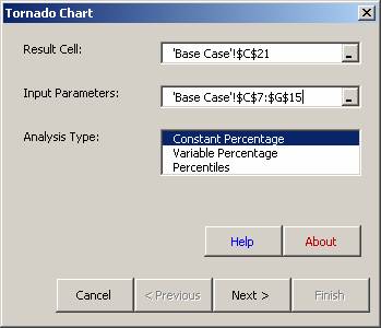
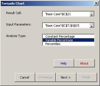
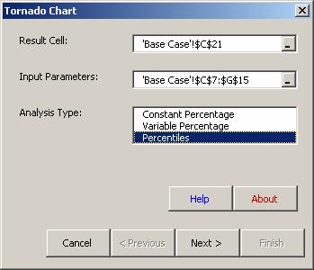
Select Sensitivity Toolkit – Tornado Chart.
Specify the cell address for the Result, Profit, in cell C21.
Specify a range for the Input Parameters, C7:G15 (blank cells are ignored).
Choose Constant Percentage for Analysis Type.
Click on Next.
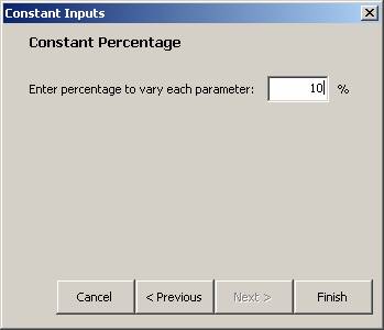
Next select the percentage amount to vary each parameter.
Click on Finish.
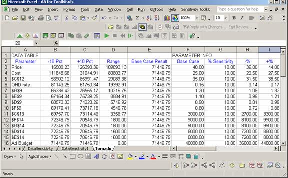
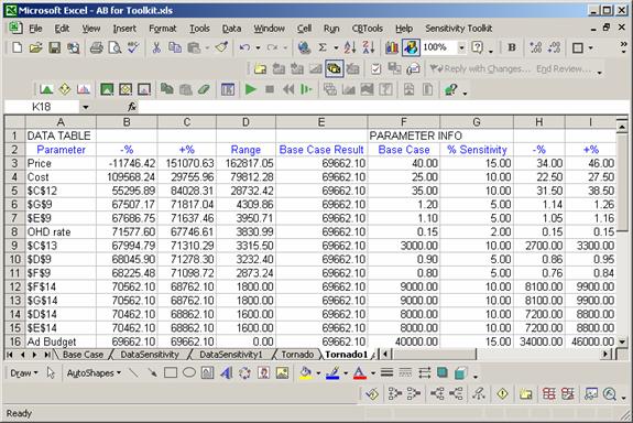
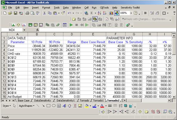
The results consist of a table of the base case values and the high and low results for each input, and the Tornado Chart.
Variable Percentage Option
Procedure:
Select Sensitivity Toolkit – Tornado Chart.
Specify the cell address for the Result, Profit, in cell C21.
Specify a range for the Input Parameters, C7:G15 (blank cells are ignored).
Choose Variable Percentage for Analysis Type.
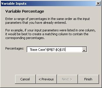
Click on Next.
Specify the percentages for each input parameter. It is best to create a separate range in the spreadsheet for these percentages. For example, we have entered the required percentages in M7:Q15.
Click Finish.
The results consist of a table of the base case values and the high and low results for each input, and the Tornado Chart.
Percentile Option
Procedure:
Select Sensitivity Toolkit – Tornado Chart.
Specify the cell address for the Result, Profit, in cell C21.
Specify a range for the Input Parameters, C7:G15 (blank cells are ignored).
Choose Percentiles for Analysis Type.
Click on Next.
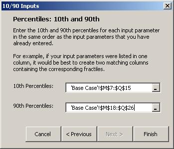
Specify a range of the 10th and 90th percentiles for each input parameter. It is best to create two separate ranges in the spreadsheet for these percentiles. For example, we have entered the required percentages in M7:Q15 and M18:Q26, respectively.
Click Finish.
The results consist of a table of the base case values and the high and low results for each input, and the Tornado Chart.
Purpose: Solver Sensitivity is used to trace the effects on the optimal solution of changes in one (or two) inputs. It calls on Solver to optimize a spreadsheet model for each of the input values specified by the user. It reports the value of the objective function and the unit change in the objective for each value of the input parameter. It also can report any other values in the spreadsheet, including the values of the decision variables.
Options:
One-way table: specify one input parameter
Two-way table: specify two input parameters
Examples:
One-way Solver Sensitivity
Procedure:
Make sure that Solver has been run at least once on the model.
Select Sensitivity Toolkit – Solver Sensitivity.
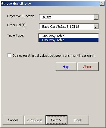
Specify the cell address for the Objective Function, Profit, in cell C21. (Normally, this selection will have been made automatically.)
Specify any other cells to include in the table; in this case we will include the decision variables in D18:G18.
Choose One-Way Table.
Click on Next.
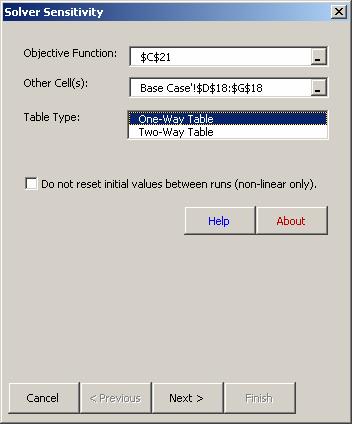
Note: The check box can be used to control the initial values of the decision variables in nonlinear optimization problems. When this box is NOT checked, each successive run of Solver will start with the values of the decision variables in the spreadsheet at the start of the sensitivity run. If this box IS checked, each successive run will use the final decision variables from the previous run as its starting values.
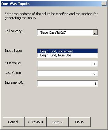
Select the input parameter, Price, in cell C7.
Specify the range over which to vary Price: 30 to 50 in steps of 1.
Click on Finish.
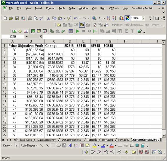
The results consist of a table with the value of the input parameter, the value of the objective function, the unit change in the objective function per unit change in the input parameter, and the values of the Other Cells.
Two-way Solver Sensitivity
Procedure:
Make sure that Solver has been run at least once on the model.
Select Sensitivity Toolkit – Solver Sensitivity.
Specify the cell address for the Objective Function, Profit, in cell C21.
(Normally, this selection will have been made automatically.)
Specify any other cells to include in the table; in this case we will include the decision variables in D18:G18.
Choose Two-Way Table.
Click on Next.
Note: The check box can be used to control the initial values of the decision variables in non-linear optimization problems. When this box is NOT checked, each successive run of Solver will start with the values of the decision variables in the spreadsheet at the start of the sensitivity run. If this box IS checked, each successive run will use the final decision variables from the previous run as its starting values.
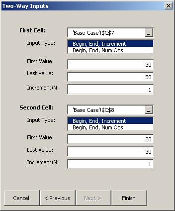
Specify the first input, Price, in cell C7, and its range of variation (30 to 50 in steps of 1).
Specify the second input, Cost, in cell C8, and its range of variation (20 to 30 in steps of 1).
Click on Finish.
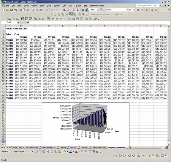
The results consist of a two-way table showing the values of the objective function for all combinations of the two input parameters. A 3D chart is also provided.
Purpose: Crystal Ball Sensitivity is used to trace the effects of changes in one (or two) inputs. It calls on Crystal Ball to run a simulation for each of the input values specified by the user, and reports the resulting values for Forecast cells.
Options:
One-way table: specify one input parameter
Two-way table: specify two input parameters
Examples:
One-way Crystal Ball Sensitivity
Procedure:
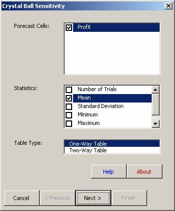
Select Sensitivity Toolkit – Crystal Ball Sensitivity.
Select the Forecast cell(s), here Profit. (Crystal Ball Sensitivity will recognize all the Forecast cells defined in the model.)
Select the Statistics to record, here the Mean. (The available statistics include the Number of Trials, Mean, Standard Deviation, Minimum, Maximum, and Mean Standard Error.)
Select One-way Table.
Click Next.
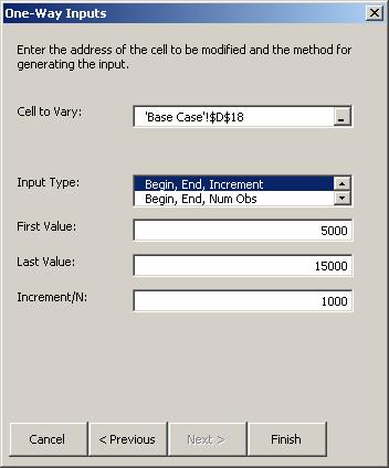
Enter the Cell to Vary, here Q1 Advertising in D18.
Specify the range over which to vary the input parameter, here 5000 to 15000 in steps of 1000.
Click on Finish.
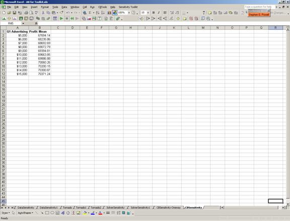
The results consist of a table with the input parameter Q1 Advertising in the first column and the mean value of Profit as estimated by simulation in the second column.
Two-way Crystal Ball Sensitivity
Procedure:
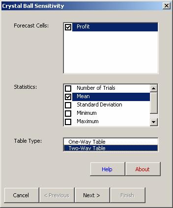
Select Sensitivity Toolkit – Crystal Ball Sensitivity.
Select the Forecast cell(s), here Profit. (Crystal Ball Sensitivity will recognize all the Forecast cells defined in the model.)
Select the Statistics to record, here the Mean. (The available statistics include the Number of Trials, Mean, Standard Deviation, Minimum, Maximum, and Mean Standard Error.)
Select Two-way Table.
Click Next.
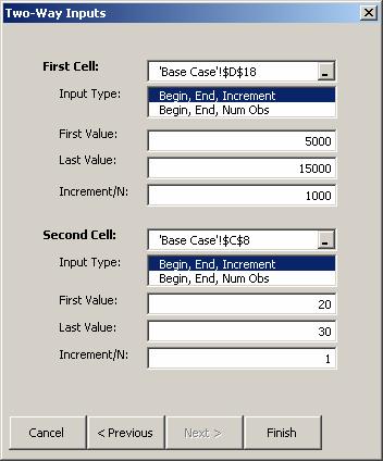
Enter the First Cell to vary, here Q1 Advertising in D18.
Specify the range over which to vary the first input parameter, here 5000 to 15000 in steps of 1000.
Enter the Second Cell to vary, here Cost in C8.
Specify the range over which to vary the second input parameter, here 20 to 30 in steps of 1.
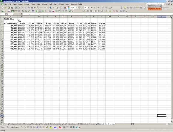
Click on Finish.
The results consist of a table with the first input parameter Q1 Advertising down the left column, the second input parameter across the top row, and the mean value of Profit as estimated by simulation in the body of the table.